Data Bars for Preliminary Analyses

Data bars are a quick way to generate informative visuals to display values in spreadsheet data. They can be used to explore data before performing additional analyses or for reports or dashboards.

They’re super easy to do.

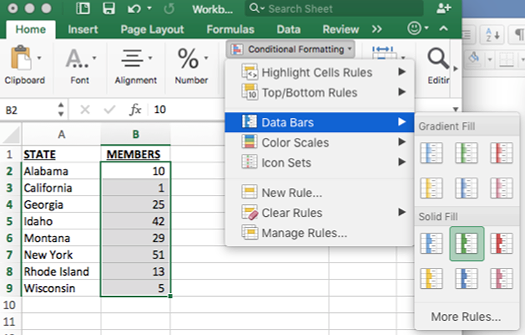
First, highlight your data and select Data Bars from the Conditional Formatting dropdown menu in the Home ribbon. There are several color options available for your bars, and you can use a solid fill or gradient.

Here’s the resulting product.

Informative, but it’s a little difficult to read the numbers when the bars are superimposed on them. Fortunately, there’s an easy fix -- you can place the bars in the column to the right of the numbers for easier reading.

First, enter a formula in column C that references the values in column B. For example, enter =B2 in cell C2 and drag the formula down to C9.

Highlight the data in cells C2 and select the More Rules option from the Data Bar drop down menu.

Check the box that says “Show data bar only” and choose your color options.

Check the box that says “Show data bar only” and choose your color options.